用 Python 理財:打造小資族選股策略-神奇的Pandas
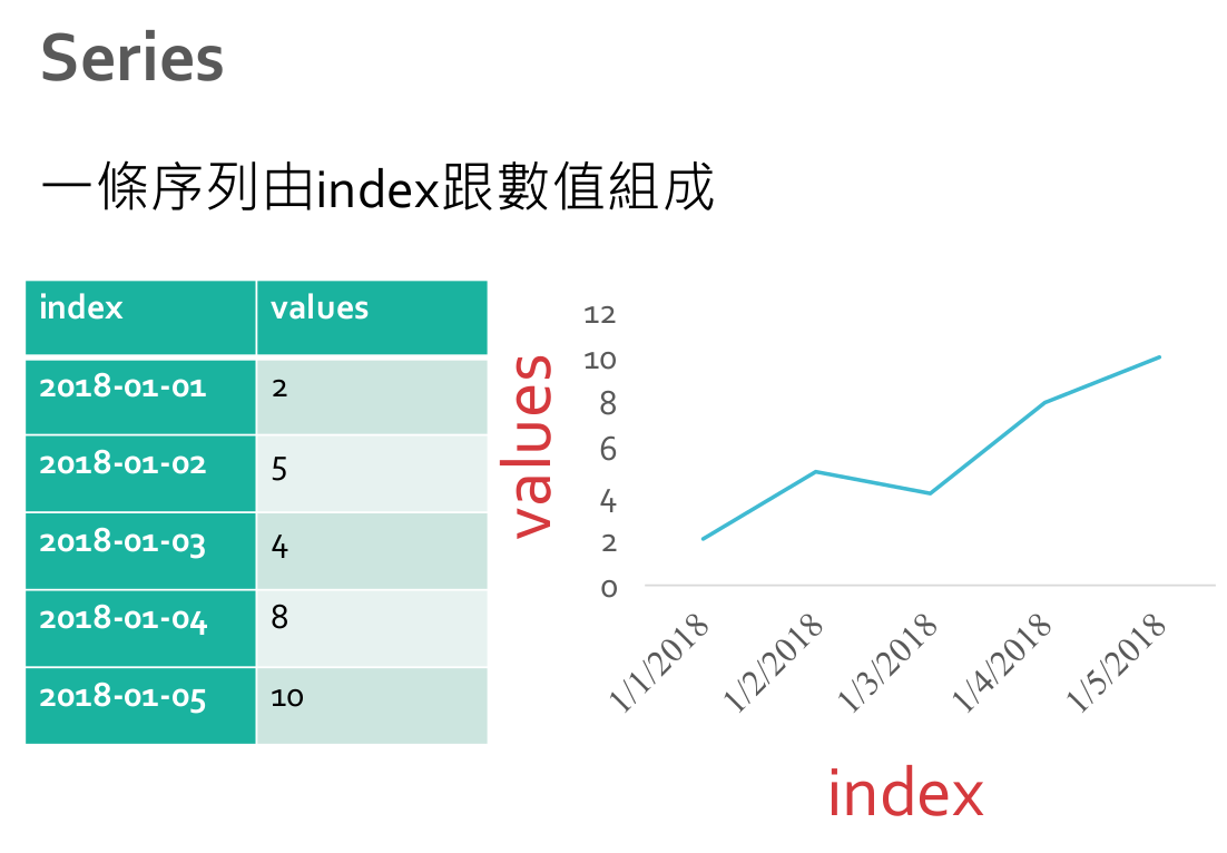
Series
語法
class pandas.Series(data=None, index=None, dtype=None, name=None, copy=False, fastpath=False)
參數
- data 純量或字典的陣列
- index 長度與 data 相同的陣列 (必須是hashable),預設值是(0, 1, 2, …, n)
- dtype str, numpy.dtype, or ExtensionDtype, optional
實例
>>> import pandas as pd
>>> s = pd.Series([1, 3, 5, np.nan, 6, 8])
>>> s
0    1.0
1    3.0
2    5.0
3    NaN
4    6.0
5    8.0
dtype: float64
>>> date = pd.date_range('20180101', periods=6)
>>> s = pd.Series([1,2,3,4,5,6], index=date)
>>> s
2018-01-01    1
2018-01-02    2
2018-01-03    3
2018-01-04    4
2018-01-05    5
2018-01-06    6
Freq: D, dtype: int64
查找
>>> s.loc['20180101'] # 輸入index
1
>>> s.loc['20180102':'2018-01-04']
2018-01-02    2
2018-01-03    3
2018-01-04    4
Freq: D, dtype: int64
>>> s.iloc[0] # 輸入第幾個
1
修改
>>> s.max()
6
>>> s.min()
1
>>> s.mean()
3.5
>>> s.std()
1.8708286933869707
>>> s.cumsum()  # 累加
2018-01-01     1
2018-01-02     3
2018-01-03     6
2018-01-04    10
2018-01-05    15
2018-01-06    21
Freq: D, dtype: int64
>>> s.cumprod()
2018-01-01      1
2018-01-02      2
2018-01-03      6
2018-01-04     24
2018-01-05    120
2018-01-06    720
Freq: D, dtype: int64
>>> s.rolling(2).sum()  # 移動窗口大小為2,且把移動窗口裡的值都加總
2018-01-01     NaN
2018-01-02     3.0
2018-01-03     5.0
2018-01-04     7.0
2018-01-05     9.0
2018-01-06    11.0
Freq: D, dtype: float64
>>> s.rolling(2).mean()
2018-01-01    NaN
2018-01-02    1.5
2018-01-03    2.5
2018-01-04    3.5
2018-01-05    4.5
2018-01-06    5.5
Freq: D, dtype: float64
>>> s + 1
2018-01-01    2
2018-01-02    3
2018-01-03    4
2018-01-04    5
2018-01-05    6
2018-01-06    7
Freq: D, dtype: int64
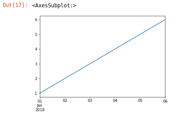
繪圖
>>> %matplotlib inline # 告訴matplotlib將圖畫在notebook上
>>> s.plot()
綜合應用
>>> s.loc[s > 3]
2018-01-04    4
2018-01-05    5
2018-01-06    6
Freq: D, dtype: int64
>>> s.loc[s > 3] = s.loc[s > 3] + 1
>>> s
2018-01-01    1
2018-01-02    2
2018-01-03    3
2018-01-04    5
2018-01-05    6
2018-01-06    7
Freq: D, dtype: int64
習題
假設某小明體重從’2018-01-01’為60公斤,由於在’2018-01-03’吃太多,導致隔天起床發現變重5公斤,
請畫出小明體重的time series
>>> weight = pd.Series(60, index=pd.date_range('2018-01-01', periods=10))
>>> weight.loc['2018-01-04':] += 5
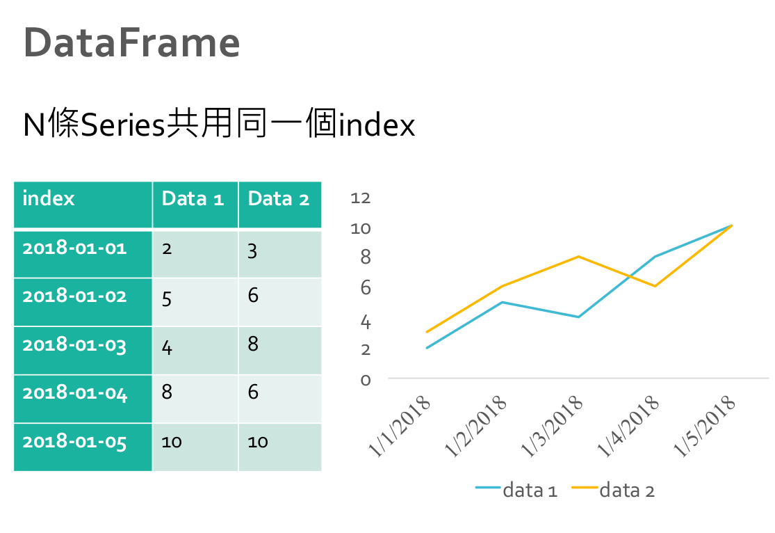
DataFrame
語法
class pandas.DataFrame(data=None, index=None, columns=None, dtype=None, copy=False)
參數
- data ndarray 或 dict
- index 長度與 data 相同的陣列 (必須是hashable),預設值是(0, 1, 2, …, n)
- columns 如果data是ndarray,那columns就代表每筆Series的名稱,預設值為(0, 1, 2, …, n);如果data是dict,那columns就是dict的key值
實例
>>> import numpy as np
>>> import pandas as pd
>>> dates = pd.date_range('20130101', periods=6)
>>> dates
DatetimeIndex(['2013-01-01', '2013-01-02', '2013-01-03', '2013-01-04',
               '2013-01-05', '2013-01-06'],
              dtype='datetime64[ns]', freq='D')

>>> df = pd.DataFrame(np.random.randn(6, 4), index=dates, columns=list('ABCD'))

>>> df
                   A         B         C         D
2013-01-01  0.469112 -0.282863 -1.509059 -1.135632
2013-01-02  1.212112 -0.173215  0.119209 -1.044236
2013-01-03 -0.861849 -2.104569 -0.494929  1.071804
2013-01-04  0.721555 -0.706771 -1.039575  0.271860
2013-01-05 -0.424972  0.567020  0.276232 -1.087401
2013-01-06 -0.673690  0.113648 -1.478427  0.524988
import pandas as pd # 引用套件並縮寫為 pd

groups = ["Modern Web", "DevOps", "Cloud", "Big Data", "Security", "自我挑戰組"]
ironmen = [46, 8, 12, 12, 6, 58]

ironmen_dict = {"groups": groups,
                "ironmen": ironmen
                }

ironmen_df = pd.DataFrame(ironmen_dict)

print(ironmen_df) # 看看資料框的外觀
#        groups  ironmen
# 0  Modern Web       46
# 1      DevOps        8
# 2       Cloud       12
# 3    Big Data       12
# 4    Security        6
# 5   自我挑戰組       58
>>> date = pd.date_range('20180101', periods=6)
>>> s1 = pd.Series([1,2,3,4,5,6], index=date)
>>> s2 = pd.Series([5,6,7,8,9,10], index=date)
>>> s3 = pd.Series([11,12,5,7,8,2], index=date)

>>> dictionary = {
    'c1': s1,
    'c2': s2,
    'c3': s3,
}

>>> df = pd.DataFrame(dictionary)
>>> df
             c1    c2    c3
2013-01-01    1    5     11
2013-01-02    2    6     12
2013-01-03    3    7      5
2013-01-04    4    8      7
2013-01-05    5    9      8
2013-01-06    6   10      2
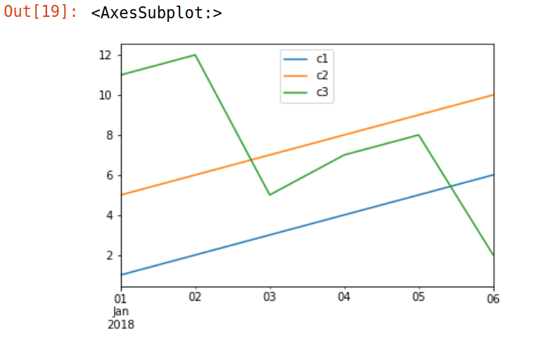
>>> %matplotlib inline
>>> df.plot()
選取
>>> df.loc['2018-01-02']
c1     2
c2     6
c3    12
Name: 2018-01-02 00:00:00, dtype: int64
>>> df.iloc[1]
c1     2
c2     6
c3    12
Name: 2018-01-02 00:00:00, dtype: int64
>>> df.loc['2018-01-02':'2018-01-05', ['c1', 'c2']]
>>> df
             c1    c2
2013-01-02    2    6
2013-01-03    3    7
2013-01-04    4    8
2013-01-05    5    9
>>> df.iloc[1:4, [0, 1]]
>>> df
             c1    c2
2013-01-02    2    6
2013-01-03    3    7
2013-01-04    4    8
>>> df.cumsum() # 每行都執行一次原本series的功能
>>> df.cumsum(axis=1)  # 每列執行cumsum()
>>> df.cumprod()
>>> df.rolling(2).mean()
>>> df.drop('c1', axis=1) # 刪除c1行
用pandas預測你的人生財務曲線
import pandas as pd
import random
%matplotlib inline
def asset_prediction(起始資金 ,起始年紀,
    每月薪水 ,
    薪水漲幅 ,
    年終獎金 ,
    每月開銷 ,
    每月房租 ,
    退休年齡 ,
    投資部位,
    投資年利率,
    買房價格,
    買房頭期款,
    買房年紀,
    房貸利率,
    貸款年數,):

    def AnnualSalary_Calculate(arr, ratio, work_year):
        ret = [arr.iloc[0]]
        for _ in arr[1:work_year]:
            ret.append(ret[-1] * ratio)
        for _ in arr[work_year:]:
            ret.append(0)
        return pd.Series(ret, 預測時段)

    預測時段 = range(起始年紀, 100)
    每年淨額 = pd.Series(0, index=預測時段)
    每年淨額.iloc[0] = 起始資金
    年薪 = pd.Series(0, index=預測時段)
    年薪.iloc[0] = 每月薪水 * (12 + 年終獎金)
    年薪 = AnnualSalary_Calculate(年薪, 薪水漲幅, 退休年齡-起始年紀)
    #年薪.plot()
    每年淨額 += 年薪
    每年淨額 -= (每月開銷 + 每月房租) * 12


    def compound_interest(arr, ratio, return_rate):
        ret = [arr.iloc[0]]
        for v in arr[1:]:
            ret.append(ret[-1] * ratio * (return_rate/100 + 1) + ret[-1] * (1 - ratio) + v)
        return pd.Series(ret, 預測時段)

    買房花費 = pd.Series(0, index=預測時段)
    買房花費[買房年紀] = 買房頭期款
    買房花費.loc[買房年紀:買房年紀+貸款年數-1] += (買房價格 - 買房頭期款) / 貸款年數

    欠款 = pd.Series(0, index=預測時段)
    欠款[買房年紀] = 買房價格
    欠款 = 欠款.cumsum()
    欠款 = 欠款 - 買房花費.cumsum()
    利息 = 欠款.shift().fillna(0) * 房貸利率 / 100


    房租年繳 = pd.Series(每月房租*12, index=預測時段)
    房租年繳.loc[買房年紀:] = 0

    每年淨額_買房 = pd.Series(0, index=預測時段)
    每年淨額_買房.iloc[0] = 起始資金
    每年淨額_買房 += 年薪
    每年淨額_買房 -= (每月開銷*12 + 房租年繳 + 利息 + 買房花費)


    pd.DataFrame({
        #'no invest, no house': 每年淨額.cumsum(),
        'invest, no house': compound_interest(每年淨額, 投資部位, 投資年利率),
        #'no invest, house': 每年淨額_買房.cumsum(),
        'invest, house': compound_interest(每年淨額_買房, 投資部位, 投資年利率),

    }).plot()


    import matplotlib.pylab as plt
    plt.ylim(0, None)

    print('月繳房貸', (買房價格 - 買房頭期款) / 貸款年數 / 12)
    print('利息', 利息.sum() / 貸款年數)
    print('')

import ipywidgets as widgets
widgets.interact(asset_prediction,
    起始資金=widgets.FloatSlider(min=0, max=300, step=10, value=300),
    起始年紀=widgets.IntSlider(min=0, max=100, step=1, value=35),
    每月薪水=widgets.FloatSlider(min=0, max=20, step=0.1, value=5.8),
    薪水漲幅=widgets.FloatSlider(min=1, max=2, step=0.01, value=1.02),
    年終獎金=widgets.FloatSlider(min=0, max=10, step=1, value=2),
    每月開銷=widgets.FloatSlider(min=0, max=20, step=0.2, value=3),
    每月房租=widgets.FloatSlider(min=0, max=20, step=0.5, value=1.5),
    退休年齡=widgets.IntSlider(min=0, max=100, step=1, value=65),
    投資部位=widgets.FloatSlider(min=0, max=1, step=0.1, value=0.7),
    投資年利率=widgets.FloatSlider(min=0, max=20, step=0.5, value=5),
    買房價格=widgets.IntSlider(min=100, max=2000, step=50, value=1000),
    買房頭期款=widgets.IntSlider(min=100, max=2000, step=50, value=300),
    買房年紀=widgets.IntSlider(min=20, max=100, step=1, value=40),
    房貸利率=widgets.FloatSlider(min=1, max=5, step=0.1, value=2.4),
    貸款年數=widgets.IntSlider(min=0, max=40, step=1, value=25)
)